Professor Dr Udo Kebschull and Professor Dr Volker Lindenstruth, from Goethe-University and the Frankfurt Institute for Advanced Studies, discuss the multifaceted technical requirements of the ALICE experiment at CERN.
The ALICE experiment at CERN’s Large Hadron Collider (LHC) is optimised for studying heavy-ion collisions, which will occur 50,000 times per second during the LHC Run 3. These high-energy collisions create a state of matter known as the quark-gluon plasma, first existing a few microseconds after the Big Bang.
To gain insights into the characteristics of the QGP, ALICE measures nearly all the thousands of particles originating from this plasma, utilising various detectors, including the Time Projection Chamber (TPC), the Inner Tracking System (ITS), the Transition Radiation Detector (TRD), and the Time-Of-Flight (TOF) detector, to name a few. These detectors measure segments of a particle trajectory passing through the experiment. Specific, dedicated software has been developed to reconstruct and identify the track from these smaller track fragments, which is used further to fully reconstruct the particle.
ALICE weighs approximately 10,000 tonnes. It is 26m long, 16m high, and 16m wide and is located 56m below ground. It operates a solenoidal magnet for particle tracking and a dipole magnet in the forward region. The solenoidal magnet alone weighs 7,800 tons. When in operation, ALICE requires about 10 MW of power. It implements about 18 million sensors, which are read out digitally in constant walk. During beam time, these sensors measure the 50 kHz interactions.
For the LHC Run 3, ALICE is employing a new concept, where all detectors are continuously read out. Baselines are suppressed by comparing the measured signals with defined thresholds. Each of the millions of sensors are corrected for baseline, gain, etc. Following this, the emerging particles are reconstructed online. This requires the processing of a data stream exceeding 600 GB/s. It is paramount that the reconstruction algorithms are efficient and, at the same time, highly precise.
Computing requirements for the EPN system
To measure and identify the particles produced in the collision, various detectors providing different particle properties, are utilised. The ITS, for instance, is used to precisely identify the primary collision vertex from which most particles emerge.
Furthermore, it allows the identification of secondary vertices, resulting from the decay of short-lived particles. The TPC measures the momentum and energy loss of the particles, with the latter allowing the extraction of the particle’s species. The TOF provides time-of-flight information and thereby the velocity of the particles, which again allows calculation of the particle’s mass, based on the measured momentum.
To first order, the charged particle trajectories have the form of a helix with decreasing radius due to the energy loss experienced while traversing the detectors. However, there are several distortion and scattering effects that disturb this ideal trajectory form. Additionally, there are noise hits and space points due to crossing particle tracks, which are hard to disentangle. All these factors must be a consideration in the reconstruction software. See Fig. 1 above.
The ALICE sub-detectors measure different space-time coordinates along a particle’s trajectory. Track candidates are initially identified via tracklets, which are then extended by adding detector hits. This process is not unambiguous and can lead to fake tracks, which must be kept to a minimum. Convoluted clusters must be identified and deconvoluted. All distortions in the detector, for instance in the TPC, which are caused by space charges need to be accounted for and corrected. Many operational parameters of the detectors change during the measurement and need to be constantly determined and updated so that the online reconstruction always relies on the most accurate calibration.
The goal is, of course, to reconstruct the majority of particles traversing the detector. In the case of the TPC, ALICE reconstructs about 98% of all particles with a momentum larger than 0.5 GeV/c. The reconstruction is based on a highly efficient algorithm that was developed by the authors and colleagues, which employs a track search algorithm that uses cellular automata and a Kalman filter for precise reconstruction of the helical trajectory.
When all trajectories of all detectors have been processed, the various tracks have to be matched between the detectors, thereby creating the full particle trajectory through ALICE. This process naturally elongates the tracks and therefore further increases the accuracy. There is, however, quite some combinatorial background which is compute-time intense and must be kept to a minimum. Once this step is complete, a collision is fully reconstructed and physics analyses can be conducted based on the measured particle properties.
Overall system architecture
The continuous data stream of all detector sensors is zero suppressed and grouped into time slices. There is a centralised clocking scheme, which allows the synchronisation of all sensors so that all heartbeat frames cover the exact same time interval in real time (89.4 µs). FPGA receiver cards, located on the First Level Processors (FLPs), receive the individual heartbeat frames from the connected optical links and combine them into one time frame, consisting of up to 120 consecutive heartbeat frames.
The software to reconstruct the various collisions contained in a time frame is very complex, thus a decision was taken to process one time frame on one server. Consequently, the various time frames are combined on one server each of the Event Processing Node (EPN) farm, which constitutes a many-to-one scenario. This requires a data distribution scheme where all FLPs simultaneously transfer the time slices, at all times, to different EPN servers in such a way that each EPN server receives a complete time frame.
To summarise, it takes 200 steps for the 200 FLP servers to transfer one time frame to an EPN server. This is implemented by a scheduler which orchestrates the data streams and accounts for nodes that may complete a time frame earlier than others. The scheduled transfer scheme provides a congestion-free network. There is enough reserve bandwidth to allow the storage of the output data which happens at 1 Tb/s.
Hardware architecture
To provide a flexible infrastructure for the complex processing requirements, outlined above, a hybrid cluster is deployed. The first stage is the FLPs, which are central processing unit (CPU) servers, hosting the 477 FPGA PCIe coprocessor cards, which also terminate the 9000 optical detector links. The FLPs are connected to the processing (EPN) farm implementing 250 servers with two 32-core AMD Rome CPUs and 8 AMD MI50 graphics processing units (GPUs) with 32 GB memory each. Each server has 512 GB of main memory to implement adequate queueing space. All nodes of the system are networked with an InfiniBand fat tree at 100 Gb/s. The EPN farm is connected to a 100 PB mass storage, with two redundant 1.6 Tb/s Ethernet links, which are directly coupled to the InfiniBand core. The storage, located about 5km away, can absorb an entire heavy-ion data taking run. The EPN farm also houses a few additional generic servers for cluster maintenance, such as logging, access control, etc.
Software architecture
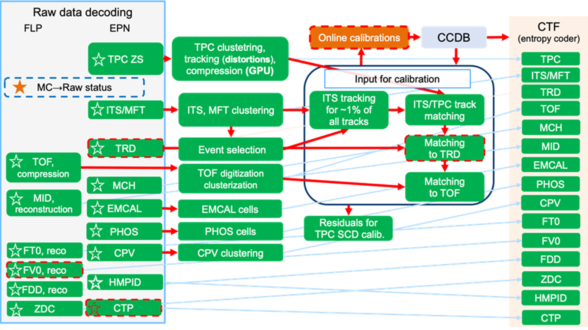
The major software modules of the online reconstruction are sketched in Fig. 2. The raw detector data is received by the FLPs using the PCIe FPGA coprocessors. There, some raw data formatting, and decoding is performed. All other operations are performed on one EPN node for each particular time frame. The majority of the EPN software (95%) is executed on the GPUs.
The first step of the reconstruction is the determination of the signal hits in the various detectors (clusterisation, cell detection). More than 90% of the compute time is consumed by the TPC reconstruction. The next step is the determination of tracks, which are derived from the clusters. This is a rather challenging step, as there is a huge combinatorial background, but this is mitigated using highly optimised algorithms based on a two-stage approach. Firstly, tracklets are identified using a cellular automaton, which has the advantage of being able to identify a large number of tracks in parallel, utilising the many compute cores of the GPU. In the second step, the tracklets are fitted using a Kalman filter, which allow us to run stably using only a single-precision floating-point format.
During the testing phase, the optimised algorithm outperformed the state-of-the-art by a factor of 10,000 on the same hardware. However, an additional complication arises from the much higher interaction rates of the upcoming LHC Run 3. Under these conditions, space charge piles up inside the TPC, leading to distortions of the tracks of up to 20cm, where the measurement accuracy is about 400µm. The interaction rate is constantly measured, and the corresponding space charge accumulated. With the knowledge of the space charge, the distortion can be corrected. In total, the TPC track finding efficiency is beyond 98% and the rate of fake tracks is below 2%.
In a next step, the TPC tracks are matched to those of the ITS detector, which is the innermost detector of ALICE, and the resulting tracks are then matched to the TRD and TOF detectors. The matching between the TPC and TRD is particularly useful for fine-tuning the calibration, since both are drift detectors, but with their drift direction orthogonal to each other.
The calibration step is an essential functionality in the software, as it is required to reconstruct the tracks but also tracks are required to fine-tune the calibration. Since the full analysis is done online, it has to be accurate, otherwise data could be discarded or tracks not found, biasing the measurement.
The final step of the online software is to compress the resulting data. One year of running is expected to produce about 100 PB of compressed data. This amplifies the importance of data compression. Various procedures are being used, including entropy encoders.
CPU usage and vectorization
Due to the use of multiple cores, which are optimal for multithreaded programmes and vectorization, the single-core performance of processors has improved. To date, CPU cores implement 512-bit vector registers, allowing the execution of, for example, 16 single-precision floating-point operations simultaneously using one machine instruction by, for instance, adding the individual vector elements of two vector registers. Such operations are well suited for any kind of matrix operation. It should be noted that a lack of vector instructions reduces the utilised peak performance of a CPU core to 1/16 of its capabilities.
However, for peak vectorization utilisation, the data structures in memory must be organised accordingly. For instance, arrays of structures lead to scatter/gather operations, which are very costly and slow. On the other hand, structures of arrays allow these long vector registers to be filled with one-load operation, simultaneously fetching all 16 elements. Note that the size of a 512-bit vector register corresponds to a cache line. Consequently, the aligning of the data structures with the cache granularity is also an important factor. The auto vectorisation functionality of compilers cannot repair what is broken in the source code. For example, a data-dependent if-instruction within a loop can prevent the loop unrolling and vectorization functionality of the compiler. Therefore, it is paramount that vectorization is kept in mind when designing the algorithm and the programme.
Since memory misses caused by cache misses are very expensive and often lead to stalls in the CPU core’s execution pipeline, it is important to pay attention to the cache efficiency of the processor. Considering that a single-cache miss can take as long as the execution of more than 800 instructions, often the better strategy is to recalculate a value rather than fetching it from memory.
Unfortunately, in the past, the software trend was opposite to this, where iterations of simple compute sequences were iteratively executed on common block memory regions. To fully utilise modern CPUs, such software needs to be rewritten.
FPGA coprocessors
The raw data from the detectors is read out via fibre-optic lines and a special protocol developed at CERN, for which a suitable firmware implementation exists. Since FPGAs have several dozen fast multi-gigabit transceivers in a single chip, they are well suited for taking over the data in the cluster. If the data is available in the FPGA, it is appropriate to perform the first bit-level calculations directly in the FPGA. Such calculations are, for example: noise reduction, common-mode correction, sorting, and normalisation of the raw data.
This is where FPGAs standout: they are particularly suitable for data streams, bit-level operations and long sequences of operations corresponding to a fixed number of loop passes, where sequential operations are mapped onto the area of the FPGA. A suitable programming paradigm is dataflow programming, for which various high-level compilers already exist. After these computational steps, the data is transferred to the computational node via a PCIe interface.
GPU coprocessors
GPUs implement, in comparison to CPUs, several thousands of compute cores together with very large register files. The memory bandwidth, exceeding 1 TB/s, is equally high. Data is exchanged with the host memory using PCIe 4.0 at more than 50 GB/s. Typically, roughly 64 cores are organised in compute engines where they operate in a vector-like fashion, always executing the same instruction but operating on different registers. Therefore, GPUs are also called ‘single instruction, multiple thread’ (SIMT) in comparison to the vector instructions of processors being called ‘single instruction, multiple data’ (SIMD). SIMT is more flexible than SIMD, thus properly vectorised software is well suited to run on GPUs.
Special care needs to be taken with respect to data structures, particularly in the case of vector instructions. However, scatter/gather instructions are even more expensive here. GPUs try to coalesce the load and store instructions of the different compute cores together. Scatter/gather typically breaks that functionality, dramatically slowing down the memory access.
Given the large number of compute cores, a high degree of parallelism is mandatory to exploit the compute performance of the GPU. Another important feature of GPUs is that they can switch the context within one clock cycle. Therefore, if the processing stalls on one instruction stream, the GPU switches automatically to the next, hiding the latencies, for example due to cache misses. However, this requires even more tasks to be available for computation.
The third performance-relevant element is the transfer of the data to and from the host memory. Although GPUs can perform random access reads and writes directly to the host memory, those instructions are particularly slow and therefore expensive. A good solution is to copy a larger memory block for the subsequent processing to the GPUs local memory and then later copy the processed result back. Ideally these three steps can happen simultaneously when the result of the previous processing is sent back to the host memory, the current is being processed, and the data for the next step is fetched. GPUs support such simultaneous operations using their powerful DMA engines. However, the algorithm must be implemented accordingly.
The ALICE event reconstruction algorithms implement all features highlighted above. It almost exclusively uses single-precision floating-point operations, utilising a much higher GPU compute performance. Initially, the GPU utilisation was rather low. This was caused by the fact that the various tracklets have different lengths. Consequently, one long tracklet in a compute engine would leave all other cores with shorter tracklets in a stall. Therefore, longer tracklets were broken up into several shorter tracklets, which were at first processed independently. To achieve the highest possible utilisation, the different compute engines are assigned tracklets dynamically by a scheduler. A postprocessor then merges these tracklets to the long tracks in the detector. The incurred extra work is overcompensated by the higher utilisation of the GPU.
Performance and results
There are a variety of performance numbers for the described reconstruction software, of which we present a selection here. First, the processing time of a data set depends linearly on the number of clusters to be processed. The AMD MI50 GPU replaces about 90 CPU cores (AMD Rome 3.3 GHz). This means that a CPU-only compute farm would have cost seven times the amount of the hybrid GPU/CPU cluster. Concerning the particle reconstruction, the transverse and longitudinal position resolution inside the TPC is 0.6 and 0.8mm, respectively, depending on the momentum of the particle. The relative transverse momentum (pT) resolution varies from 1% (pT < 1GeV/c) to 10% (pT < 20GeV/c). The track reconstruction efficiency is better than 95% for pT < 0.2GeV/c.
Conclusion
ALICE is the first LHC experiment to use GPUs to the fullest extent possible. This design resulted in a cost saving of $36m for the EPN compute farm. The use of GPUs also provides a significant reduction of power consumption by the EPN compute farm. Therefore, this system is both economical and ecological. Over 95% of the reconstruction software runs on GPUs. The CPUs mostly perform data orchestration and house-keeping functionalities. The next steps, which are currently being pursued, are the adaptation of the remaining offline or asynchronous software to also use GPUs to the largest extent possible.